Eigendecomposition and Hodge decomposition
In this tutorial, we will show how to perform the eigendecomposition and
the Hodge decomposition of a SC using the decomposition module.
Eigendecomposition
We can represent the signals of different orders over bases built with the eigenvectors of the higher-order Laplacian matrices. Thus, the eigendecomposition of the Hodge Laplacians is defined as
where \(\mathbf{U}_k\) is an orthonormal matrix that collects the eigenvectors and \(\mathbf{\Lambda}_k\) is a diagonal matrix with the associated eigenvalues. The Hodge decomposition establishes a correspondence between \(\mathbf{U}_1\) and the three orthogonal subspaces, that is, the eigenvectors of \(\mathbf{U}_1\) fully span the three orthogonal subspaces, namely gradient, curl, and harmonic, given by the Hodge decomposition. Given the 1-Hodge Laplacian of a simplicial complex
the following holds:
Gradient eigenvectors \(\mathbf{U_G} = [ \mathbf{u_{G, 1}} \dots \mathbf{u}_{\mathbf{G}, N_\mathbf{G}}] \in \mathbb{R}^{N_1 \times N_{\mathbf{G}}}\) of \(\mathbf{L}_{1,l}\), associated with their corresponding nonzero eigenvalues, span the gradient space \(im(\mathbf{B}_1^\top)\) with dimension \(N_\mathbf{G}\).
Curl eigenvectors \(\mathbf{U_C} = [ \mathbf{u_{C, 1}} \dots \mathbf{u}_{\mathbf{C}, N_\mathbf{C}}] \in \mathbb{R}^{N_1 \times N_{\mathbf{C}}}\) of \(\mathbf{L}_{1,u}\), associated with their corresponding nonzero eigenvalues, span the curl space \(im(\mathbf{B}_2)\) with dimension \(N_\mathbf{C}\).
Harmonic eigenvectors \(\mathbf{U_H} = [ \mathbf{u_{H, 1}} \dots \mathbf{u}_{\mathbf{H}, N_\mathbf{H}}] \in \mathbb{R}^{N_1\times N_{\mathbf{H}}}\) of \(\mathbf{L}_{1}\), associated with their corresponding zero eigenvalues, span the harmonic space \(ker(\mathbf{L}_1)\) with dimension \(N_\mathbf{H}\).
The eigendecomposition of a SC can be calculated in the following way for harmonic, curl and gradient components:
>>> from pytspl import load_dataset
>>>
>>> sc, coordinates, _ = load_dataset("paper")
>>> u_h, eigenvals_h = sc.get_component_eigenpair(component="harmonic")
>>> u_c, eigenvals_c = sc.get_component_eigenpair(component="curl")
>>> u_g, eigenvals_g = sc.get_component_eigenpair(component="gradient")
>>>
>>> print("Eigenvalues:", eigenvals_h)
>>> print("Harmonic component:", u_h)
Eigenvalues: [7.10542736e-15]
Harmonic component:
[[ 0.06889728]
[ 0.13779456]
[-0.20669185]
[ 0.06889728]
[-0.34448641]
[ 0.55117825]
[-0.55117825]
[-0.36745217]
[-0.18372608]
[ 0.18372608]]
To plot the eigenpairs for a component, we can use the following code:
>>> from pytspl import SCPlot
>>>
>>> scplot = SCPlot(simplicial_complex=sc, coordinates=coordinates)
>>> scplot.draw_eigenvectors(component="gradient")
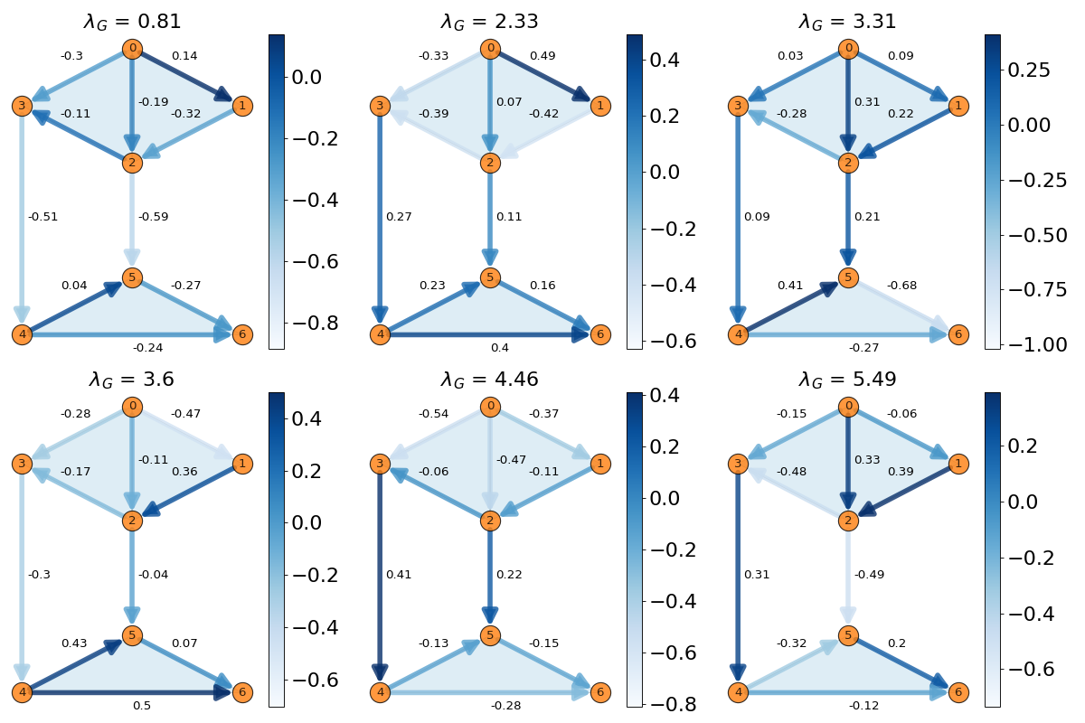
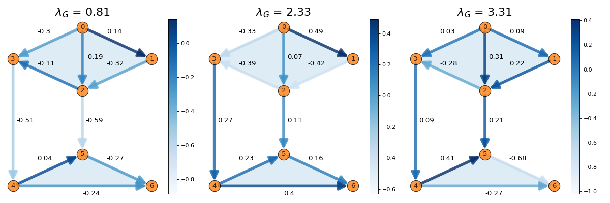
We can also plot the selected indices of the eigenvectors:
>>> indices = [0, 1, 2]
>>> scplot.draw_eigenvectors(component="gradient", eigenvector_indices=indices)
Hodge decomposition
The Hodge decomposition states that the space of \(k\)-simplex signals can be decomposed into three orthogonal subspaces that can be written as
where \(im\) is the image space and \(ker\) is the kernel space of the respective matrices. The subspace \(im(\mathbf{B}_{k+1})\) is known as the gradient subspace, \(im(\mathbf{B}_{k}^\top)\) as the curl subspace, and \(ker(\mathbf{L}_k)\) as the harmonic subspace. Therefore, we can decompose any edge flow \(\mathbf{f} \in \mathbb{R}^{N_1}\) into the orthogonal components
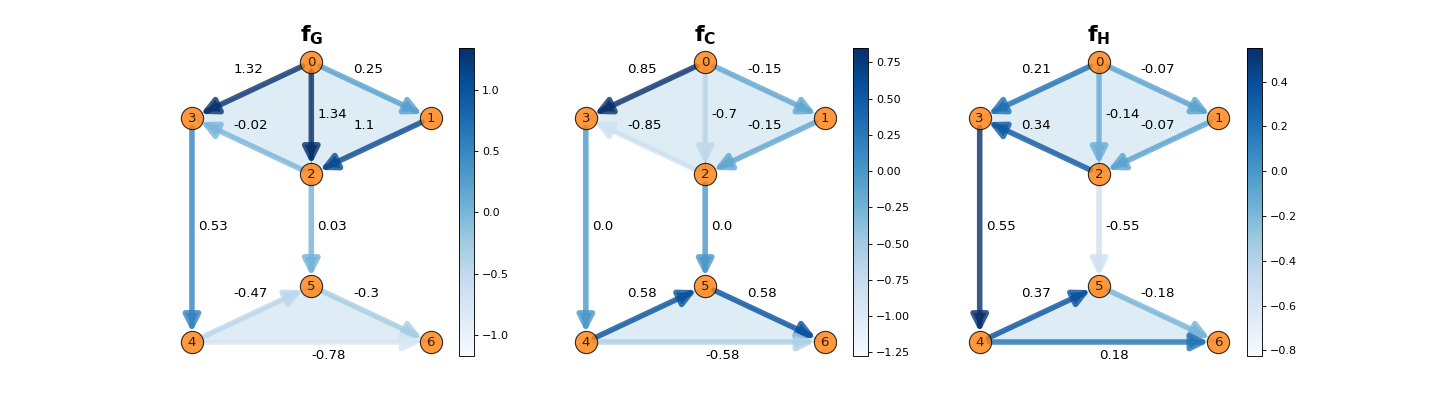
where \(\mathbf{f}_G\) is the gradient component \(\mathbf{f}_G \in im( \mathbf{B}_1^\top )\), \(\mathbf{f}_C\) is the curl component \(\mathbf{f}_C \in im( \mathbf{B}_2 )\), and \(\mathbf{f}_H\) is the harmonic component \(\mathbf{f}_H \in ker( \mathbf{L}_1 )\). By decomposing the signal into three different components, we can extract the different properties of the flow. For instance, we can study the effect of an external source or sink by extracting the gradient component of the edge flow.
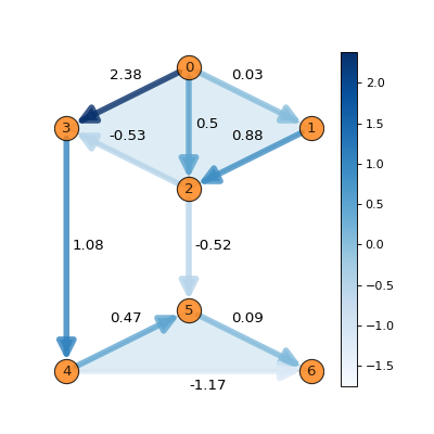
The Hodge decomposition of an edge flow can be calculated using the same module. First, we need to create a synthetic flow:
>>> fig, ax = plt.subplots(figsize=(5, 5))
>>>
>>> synthetic_flow = np.array([0.03, 0.5, 2.38, 0.88, -0.53, -0.52, 1.08, 0.47, -1.17, 0.09])
>>> scplot.draw_network(edge_flow=synthetic_flow, ax=ax)
We can get the divergence and the curl in the following way:
>>> sc.get_divergence(synthetic_flow)
array([-2.91, -0.85,  2.43,  0.77,  1.78, -0.14, -1.08])
>>> sc.get_curl(synthetic_flow)
[ 0.41 -2.41  1.73]
To get the harmonic, curl and gradient flows, we can do the following:
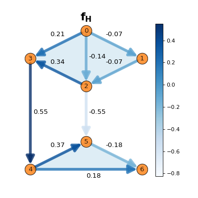
>>> f_h = sc.get_component_flow(flow=synthetic_flow, component="harmonic")
[-0.07 -0.14  0.21 -0.07  0.34 -0.55  0.55  0.37  0.18 -0.18]
>>> f_g = sc.get_component_flow(flow=synthetic_flow, component="gradient")
[ 0.25  1.34  1.32  1.1  -0.02  0.03  0.53 -0.47 -0.78 -0.3 ]
>>> f_c = sc.get_component_flow(flow=synthetic_flow, component="curl")
[-0.15 -0.7   0.85 -0.15 -0.85  0.    0.    0.58 -0.58  0.58]
Plot the harmonic, curl and gradient flows using the following code:
>>> scplot.draw_hodge_decomposition(flow=synthetic_flow, figsize=(18, 5))
To plot the harmonic flow only, we can do the following:
>>> scplot.draw_hodge_decomposition(flow=synthetic_flow, component="harmonic", figsize=(5, 5))