Introduction to Filters
PyTSPL has functional for various filters, namely Simplicial Convolutional Filters and Simplicial Trend Filters.
The Simplicial Convolutional Filters include the following filters:
Least-Squares (LS) Filter Design
Grid-based Filter Design
Chebyshev Polynomial Filter Design
Filter Designs
Given a dataset of input-output edge flow relations \(T = \{(\mathbf{f}_1, \mathbf{f}_{o, 1}), \ldots, (\mathbf{f}_{|T|}, \mathbf{f}_{o, |T|})\}\), we learn the filter coefficients by aligning the filter’s output \(\mathbf{H_1} \mathbf{f}\) with the observed output \(\mathbf{f}_o\). The filter coefficients here are learned in a data-driven manner. The optimization utilizes a mean squared error (MSE) cost function, enhanced with a regularization term \(r(\mathbf{f}_0, \boldsymbol{\alpha}, \boldsymbol{\beta})\), to prevent overfitting. The problem is formulated as:
where \(\gamma > 0\) acts as the regularization coefficient, balancing fit and complexity to improve model generalization.
We aim to design simplicial filters given a desired frequency response. First, we considered the standard least-squares (LS) filter design and following that, we consider a universal filter design that avoids the eigenvalue computation given a continuous frequency response. In particular, we consider grid-based and Chebyshev polynomial filter designs.
This tutorial will introduce Chebyshev Polynomial filter design. Tutorials for other filters
can be found under notebooks/filters. All the filters are included in the pytspl.filters
module.
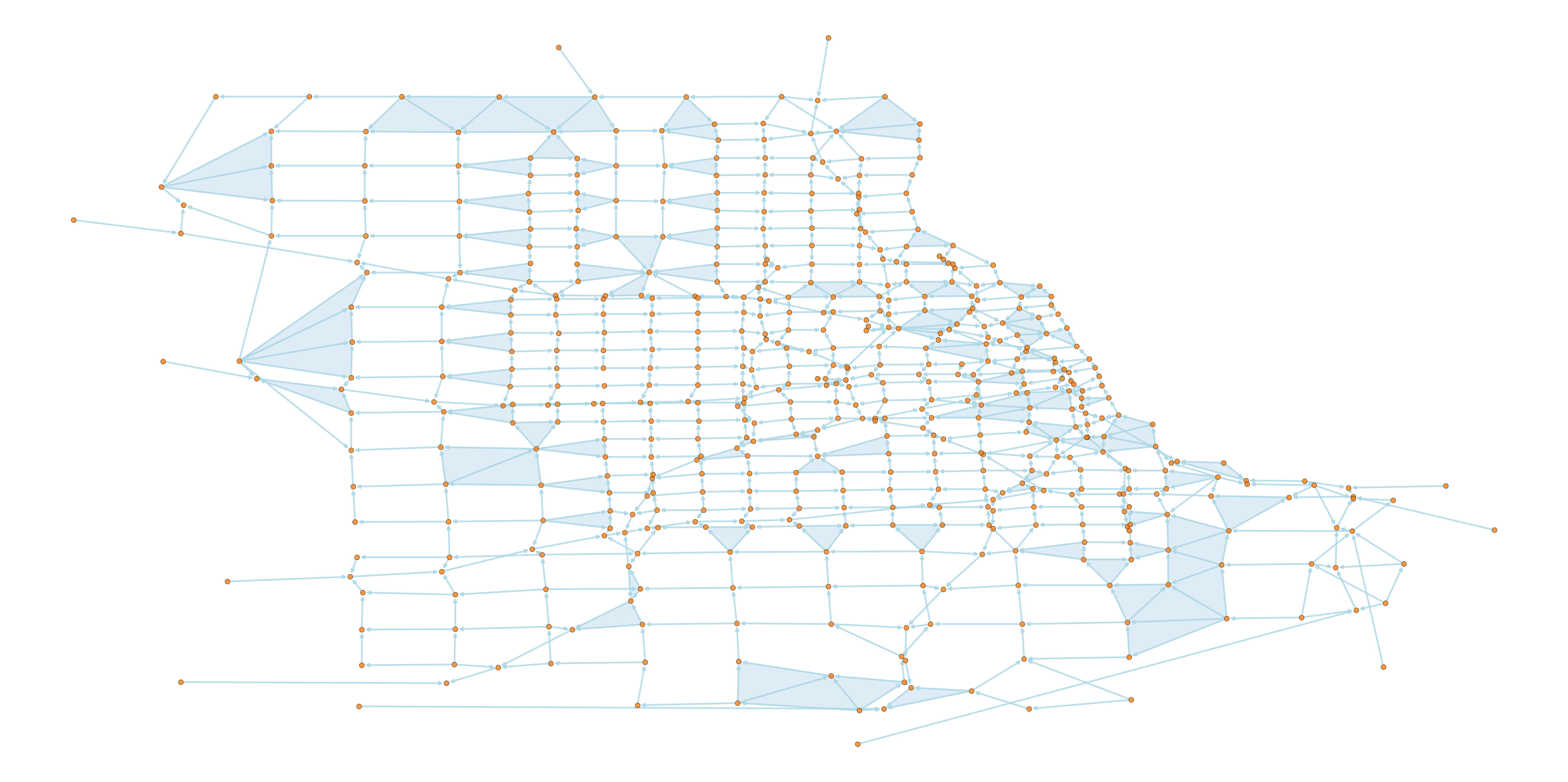
Load the chicago-sketch dataset as a simplicial complex.
>>> from pytspl import load_dataset
>>>
>>> # load the chicago-sketch dataset
>>> sc, coordinates, flow = load_dataset("chicago-sketch")
>>>
>>> # convert the flow to an numpy array
>>> flow = np.asarray(list(flow.values()))
Num. of nodes: 546
Num. of edges: 1088
Num. of triangles: 112
Shape: (546, 1088, 112)
Max Dimension: 2
Coordinates: 546
Flow: 1088
Plot the simplicial complex using the draw_network() function.
>>> from pytspl import SCPlot
>>>
>>> fig, ax = plt.subplots(1, 1, figsize=(80, 40))
>>>
>>> scplot = SCPlot(simplicial_complex=sc, coordinates=coordinates)
>>> scplot.draw_network(with_labels=False, node_size=200, arrowsize=20, ax=ax)
In the next step, we initialize the Chebyshev polynomial filter design.
>>> from pytspl.filters import ChebyshevFilterDesign
>>> chebyshev_filter = ChebyshevFilterDesign(simplicial_complex=sc)
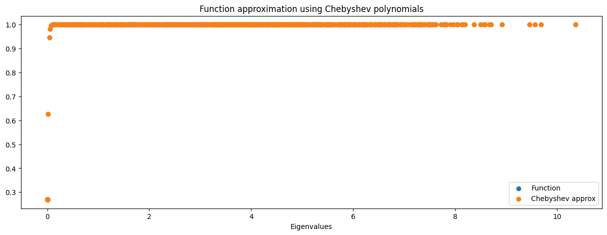
Here, we can plot the Chebyshev series approximation for a matrix \(\textbf{P}\). Additionally, we can define the number of points \(n\), the cut-off frequency, and the steepness of the filter.
>>> chebyshev_filter.plot_chebyshev_series_approx(p_choice="L1L")
To apply the filter, we need to specify the matrix \(\textbf{P}\), the component to extract, the filter size, the cut-off frequency, the steepness, and the number of points to approximate the Chebyshev series.
>>> # apply the Chebyshev filter
>>> filter_size = 50
>>>
>>> chebyshev_filter.apply(
>>>    f=flow,
>>>    p_choice="L1L",
>>>    component="gradient",
>>>    L=filter_size,
>>>    cut_off_frequency=0.01,
>>>    steep=100,
>>>    n=100
>>> )
Filter size: 0 - Error: 0.5494 - Filter error: 0.9471 - Error response: 0.9489
Filter size: 1 - Error: 0.5326 - Filter error: 0.9120610332448 - Error response: 0.9234254397938262
Filter size: 2 - Error: 0.5168 - Filter error: 0.8772 - Error response: 0.9016
Filter size: 3 - Error: 0.5023 - Filter error: 0.8427 - Error response: 0.8785
Filter size: 4 - Error: 0.4887 - Filter error: 0.8087 - Error response: 0.8527
...
Filter size: 45 - Error: 0.1495 - Filter error: 0.3583 - Error response: 0.5850
Filter size: 46 - Error: 0.1500 - Filter error: 0.3595 - Error response: 0.5851
Filter size: 47 - Error: 0.1506 - Filter error: 0.3608 - Error response: 0.5852
Filter size: 48 - Error: 0.1512 - Filter error: 0.3621 - Error response: 0.5854
Filter size: 49 - Error: 0.1512 - Filter error: 0.3621 - Error response: 0.5854
Plot the extracted component and filter error.
>>> # plot the extracted component and filter error
>>> fig, ax = plt.subplots(1, 1, figsize=(10, 5))
>>>
>>> plt.plot(chebyshev_filter.history["extracted_component_error"])
>>> plt.plot(chebyshev_filter.history["filter_error"])
>>> plt.legend(["Extracted Component Error", "Filter Error"])

Plot the approximated frequency responses of the built filter.
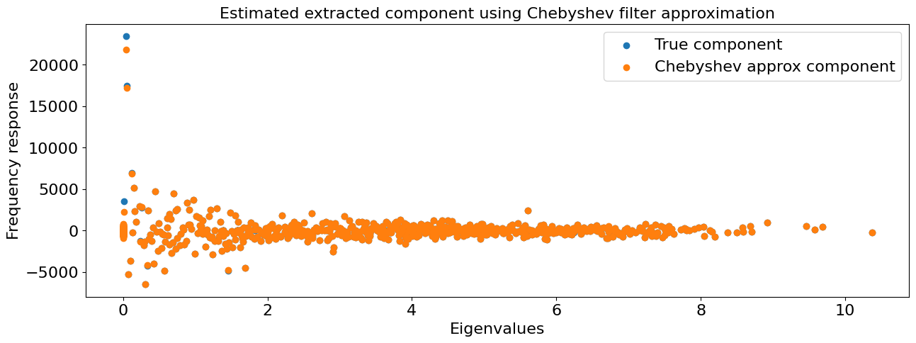
>>> chebyshev_filter.plot_frequency_response_approx(flow=flow, component="gradient")
After applying the filter, we can retrieve the history of the filter. The history contains the:
filter: the filter for each filter size
f_estimated: the estimated flow after applying the filter
frequency_responses: the frequency responses for each filter size
extracted_component_error: the extracted component error for each filter size
filter_error: the filter error for each filter size
>>> # retrieve the history of the filter
>>> cheb_filter.history
{'filter': array([[[ 9.60182326e-01,  6.52287870e-03,  6.52287870e-03, ...,
           0.00000000e+00,  0.00000000e+00,  0.00000000e+00],
         [ 6.52287870e-03,  9.60182326e-01,  0.00000000e+00, ...,
           0.00000000e+00,  0.00000000e+00,  0.00000000e+00],
         [ 6.52287870e-03,  0.00000000e+00,  9.60182326e-01, ...,
...
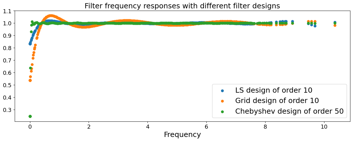
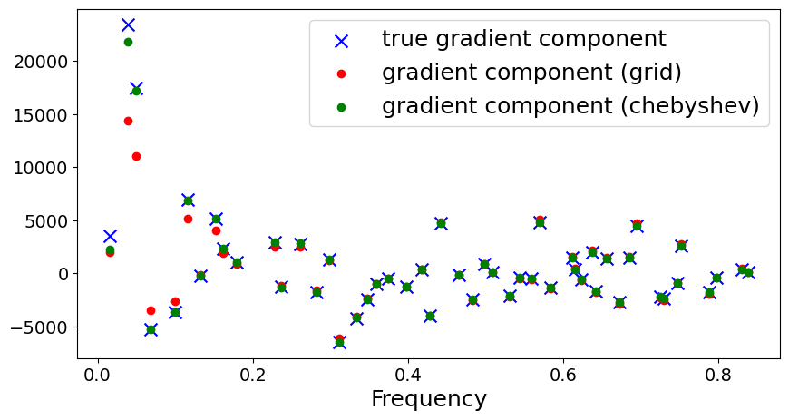
To compare the three filter designs, we applied them to the Chicago road network. For the LS-based filter design, we set a filter order of 10. Setting a low filter order avoids the ill-conditioning. For the grid-based filter design, we uniformly sampled 100 points in the interval \([0, \lambda_{G,\text{max}}]\) with \(\lambda_{G,\text{max}} = 10.8\) approximated using the power-iteration algorithm with steps = 50. The cut-off frequency \(\lambda_{0} = 0.01\) and the steep \(k = 100\) for the logistic function in the Chebyshev polynomial design.
The Chebyshev polynomial of order 50 only has a couple of frequencies smaller than 0.9 at the smallest gradient frequency. The remaining frequencies can preserve the gradient component well. The LS-based and grid-based filter designs have a poorer performance, especially at small gradient frequencies.
We can calculate the SFT of the extracted gradient component and compare it with the grid-based filter design. The comparison is plotted below. As we can see, the Chebyshev polynomial filter has a good extraction ability and performs well at very small frequencies where the grid-based design fails.
References
Yang et al. [5]
The library utilizes the chebpy Python library for Chebyshev series approximation. For more information, see the GitHub repository.