Introduction to PyTSPL

This tutorial demonstrates the basic functionality of the library. After installing the package, start by opening a Python shell, such as a Jupyter notebook, and importing PyTSPL.

Let’s begin by building a simplicial complex (SC) using the built-in dataset.

Given a finite set of vertices \(V\), a \(k\)-simplex \(S^k\) is a subset of \(V\) with \(k+1\) nodes. The face of \(S^k\) is defined as the subset of \(k\)-simplex \(S^k\) with cardinality \(k\). A coface of \(S^k\) is a simplex \(S^{k+1}\) that includes it. A simplicial complex \(\mathcal{X}\) is defined as a finite collection of simplicity satisfying the inclusion property. The inclusion property states that for any \(S^k \in \mathcal{X}\), all its faces \(S^{k-1} \subset S^k\) are also part of the simplicial complex.

Loading a SC from a dataset

Before loading a dataset, we can list the datasets that are currently available.

>>> from pytspl import list_datasets
>>>
>>> # List the available datasets
>>> list_datasets()
['barcelona',
 'chicago-regional',
 'siouxfalls',
 'anaheim',
 'test_dataset',
 'goldcoast',
 'winnipeg',
 'chicago-sketch',
 'paper',
 'forex',
 'lastfm-1k-artist',
 'wsn']

Once we load the dataset, we will receive a summary of the SC. Additionally, we will obtain the coordinates and the flow of the SC.

>>> from pytspl import load_dataset
>>>
>>> # Load the paper dataset
>>> sc, coordinates, flow = load_dataset("paper")
Num. of nodes: 7
Num. of edges: 10
Num. of triangles: 3
Shape: (7, 10, 3)
Max Dimension: 2
Coordinates: 7
Flow: 10

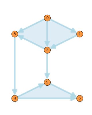
We can plot the SC using the draw_network() method of the SCPlot class. The class also includes additional methods to plot the SC with customizations. The user can plot the nodes and edges with different colors, sizes, and labels. For more details, please refer to the API documentation.

>>> from pytspl import SCPlot
>>> import matplotlib.pyplot as plt
>>>
>>> # Plot the SC using a dataset
>>> fig, ax = plt.subplots(figsize=(4, 5))
>>>
>>> sc, coordinates, flow = load_dataset("paper")
>>> scplot = SCPlot(simplicial_complex=sc, coordinates=coordinates)
>>> scplot.draw_network(ax=ax)

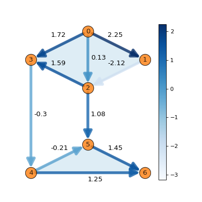
We can also plot the SC with its corresponding edge flow.

>>> # Plot the SC with edge flow
>>> fig, ax = plt.subplots(figsize=(5, 5))
>>>
>>> scplot.draw_network(edge_flow=flow, ax=ax)

To retrieve the properties of the SC, we can use the SimplicialComplex object. For example, we can obtain the adjacency matrix, incidence matrices, and the Hodge Laplacian matrices by specifying the rank as a parameter. For more details, please refer to the API documentation.

>>> # get the adjacency matrix
>>> sc.adjacency_matrix()
>>>
>>> # get the incidence matrix
>>> sc.incidence_matrix(rank=1)
>>>
>>> # get the Hodge Laplacian matrix
>>> sc.hodge_laplacian_matrix(rank=1)
array([[ 3.,  0.,  1.,  0.,  0.,  0.,  0.,  0.,  0.,  0.],
       [ 0.,  4.,  0.,  0.,  0., -1.,  0.,  0.,  0.,  0.],
       [ 1.,  0.,  3.,  0.,  0.,  0., -1.,  0.,  0.,  0.],
       [ 0.,  0.,  0.,  3., -1., -1.,  0.,  0.,  0.,  0.],
       [ 0.,  0.,  0., -1.,  3.,  1., -1.,  0.,  0.,  0.],
       [ 0., -1.,  0., -1.,  1.,  2.,  0.,  1.,  0., -1.],
       [ 0.,  0., -1.,  0., -1.,  0.,  2., -1., -1.,  0.],
       [ 0.,  0.,  0.,  0.,  0.,  1., -1.,  3.,  0.,  0.],
       [ 0.,  0.,  0.,  0.,  0.,  0., -1.,  0.,  3.,  0.],
       [ 0.,  0.,  0.,  0.,  0., -1.,  0.,  0.,  0.,  3.]])

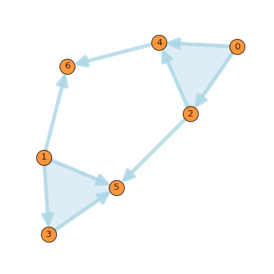
Generate a random SC

We can also generate a random SC using the generate_random_simplicial_complex() function. The function takes the number of nodes, the probability of an edge between two nodes, the seed, and the distance threshold as parameters.

>>> from pytspl import generate_random_simplicial_complex, SCPlot
>>>
>>> # generate a random SC
>>> sc, coordinates = generate_random_simplicial_complex(
>>>        num_of_nodes=7,
>>>        p=0.25,
>>>        seed=42,
>>>        dist_threshold=0.8
>>> )
>>>
>>> # plot the random SC
>>> scplot = SCPlot(sc, coordinates)
>>> scplot.draw_network()