Operations with Simplicial Complexes
This tutorial will give an overview of the algebraic operations possible with
simplicial complexes using the PyTSPL library.
Simplicial Shifting
Applying filter \(\mathbf{H}_k\) to a \(k\)-simplicial signal \(\mathbf{s}^k\) yields an output \(\mathbf{H}_k \mathbf{s}^k\) which is a shift-and-sum operation. The filter \(\mathbf{H}_k\) shifts the signal \(L_1\) times over the lower neighbourhoods and \(L_2\) times over the upper neighbourhoods. Next, the shifted results are summed together according to the corresponding coefficients. Similarly, consider an edge filter \(\mathbf{H}_1\) applied to an edge flow \(\mathbf{f}\) with the output:
where we apply different powers of the lower and upper Hodge Laplacian to the edge flow. This basic operation is known as simplicial shifting. The one-step lower and upper shifting are defined below, respectively:
Then, \(k\)-step shifting is defined as the weighted linear combination of the lower and upper shifted simplicial signals after \(k\) steps:
Let’s start by loading a dataset.
>>> from pytspl import load_dataset
>>> import matplotlib.pyplot as plt
>>>
>>> # load the paper dataset
>>> sc, coordinates, flow = load_dataset("paper")
Num. of nodes: 7
Num. of edges: 10
Num. of triangles: 3
Shape: (7, 10, 3)
Max Dimension: 2
Coordinates: 7
Flow: 10
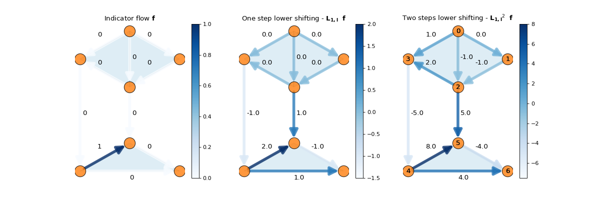
Create an indicator flow \(\mathbf{f}\).
>>> synthetic_flow = [0, 0, 0, 0, 0, 0, 0, 1, 0, 0]
In this example, we shift the signal \(L_1\) times over the lower
neighbourhoods by applying the function apply_lower_shifting()
for one and two steps.
>>> from pytspl import SCPlot
>>>
>>> # create a SC plot
>>> scplot = SCPlot(simplicial_complex=sc, coordinates=coordinates)
>>> fig, axs = plt.subplots(1, 3, figsize=(15, 5))
>>>
>>> # plot indicator flow f
>>> axs[0].set_title("Indicator flow $\mathbf{f}$")
>>> scplot.draw_network(edge_flow=synthetic_flow, ax=axs[0])
>>>
>>> # apply one step lower shifting
>>> steps = 1
>>> flow = sc.apply_lower_shifting(synthetic_flow, steps=steps)
>>>
>>> axs[1].set_title(r"One step lower shifting - $\mathbf{L_{1, l}} \ \ \mathbf{f}$")
>>> scplot.draw_network(edge_flow=flow, ax=axs[1])
>>>
>>> # apply two steps lower shifting
>>> steps = 2
>>> flow = sc.apply_lower_shifting(synthetic_flow, steps=steps)
>>>
>>> axs[2].set_title(r"Two steps lower shifting - $\mathbf{L_{1, l}}^2 \ \ \mathbf{f}$")
>>> scplot.draw_network(edge_flow=flow, ax=axs[2])
Similarly, we can apply the function apply_upper_shifting() to
shift the signal \(L_2\) times over the upper neighbourhoods.
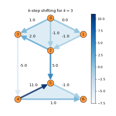
We can also apply \(k\)-step simplicial shifting using the function
apply_k_step_shifting() for \(k\) steps.
>>> # apply k-step shifting for k = 3
>>> k = 3
>>> flow = sc.apply_k_step_shifting(synthetic_flow)
>>>
>>> # plot the k-step shifting
>>> fig, ax = plt.subplots(1, 1, figsize=(5, 5))
>>> ax.set_title(r"$k$-step shifting for $k = 3$")
>>> scplot.draw_network(edge_flow=flow, ax=ax)
Simplicial Fourier Transform (SFT) and Embeddings
Given a \(k\)-simplicial signal \(s^k\), the simplicial Fourier Transform (SFT) is defined as:
which is a projection onto the eigenvectors \(\mathbf{U}_k\) where each entry \(\mathbf{s}^k_i\) represents the weight eigenvector \(\mathbf{u}^k_i\) has on \(\mathbf{s}^k\). The inverse SFT is given by:
Similarly to GFT, the eigenvalues of \(\mathbf{L}_k\) represent the notion of simplicial frequencies, but in a more meaningful way. The eigenvalues of \(\mathbf{L}_k\) measure three types of simplicial frequencies.
Gradient frequency: The magnitude of an eigenvalue \(\lambda_G\) measures the amount of total divergence in an SC. The divergence is a measure of the net flow of a signal out of a node. The gradient eigenvectors associated with large eigenvalues have a large total divergence.
Curl frequency: The magnitude of an eigenvalue \(\lambda_C\) measures the amount of total curl in an SC, i.e., rotation variation. The rotation variation is the measure of the extent of circular or rotational flow in the network. The curl eigenvectors associated with large eigenvalues have a large total curl.
Harmonic frequency: The harmonic eigenvectors \(\mathbf{U}_H\) are both divergence- and curl-free. A harmonic flow is defined as the SFT of an edge flow that has nonzero components only at the harmonic frequencies, which correspond to zero eigenvalues.
Given the three component eigenvectors, we define the three embeddings of an edge flow \(\mathbf{f} \in \mathbb{R}^{N_1}\) as follows:
These embeddings are the result of the orthogonality of these three components given by the Hodge decomposition. Using these simplicial embeddings, we can rewrite the SFT of \(\mathbf{f}\) as:
where \(\tilde{\mathbf{f}}_\mathbf{H}^\top\) is the harmonic embedding, \(\tilde{\mathbf{f}}_\mathbf{G}^\top\) is the gradient embedding, and \(\tilde{\mathbf{f}}_\mathbf{C}^\top\) is the curl embedding. Each entry of an embedding represents the weight the flow has on the corresponding eigenvector. This offers a compressed representation of the edge flow and allows us to cluster them based on their types.
Given a flow \(\mathbf{f}\), we can extract the harmonic, curl, and gradient embeddings. Such embeddings represent a compressed representation of the edge flow.
To extract the simplicial embeddings, we can use the function get_simplicial_embeddings().¨
>>> # define a synthetic flow
>>> synthetic_flow = [0.03, 0.5, 2.38, 0.88, -0.53, -0.52, 1.08, 0.47, -1.17, 0.09]
>>> # get the simplicial embeddings for harmonic, curl and gradient
>>> f_tilda_h, f_tilda_c, f_tilda_g = sc.get_simplicial_embeddings(synthetic_flow)
>>>
>>> print("embedding_h:", f_tilda_h)
>>> print("embedding_g:", f_tilda_g)
>>> print("embedding_c:", f_tilda_c)
embedding_h: [-1.00084785]
embedding_g: [-1.00061494 -1.00127703  1.00173495 -1.00287539  0.99531105  1.00412064]
embedding_c: [-1. 0.99881597  0.99702056]